Visualizing Conservative Vector Fields

Skip to main content

\(\newcommand{\vf}[1]{\mathbf{\boldsymbol{\vec{#1}}}} \renewcommand{\Hat}[1]{\mathbf{\boldsymbol{\hat{#1}}}} \let\VF=\vf \let\HAT=\Hat \newcommand{\Prime}{{}\kern0.5pt'} \newcommand{\PARTIAL}[2]{{\partial^2#1\over\partial#2^2}} \newcommand{\Partial}[2]{{\partial#1\over\partial#2}} \newcommand{\tr}{{\mathrm tr}} \newcommand{\CC}{{\mathbb C}} \newcommand{\HH}{{\mathbb H}} \newcommand{\KK}{{\mathbb K}} \newcommand{\RR}{{\mathbb R}} \newcommand{\HR}{{}^*{\mathbb R}} \renewcommand{\AA}{\vf{A}} \newcommand{\BB}{\vf{B}} \newcommand{\CCv}{\vf{C}} \newcommand{\EE}{\vf{E}} \newcommand{\FF}{\vf{F}} \newcommand{\GG}{\vf{G}} \newcommand{\HHv}{\vf{H}} \newcommand{\II}{\vf{I}} \newcommand{\JJ}{\vf{J}} \newcommand{\KKv}{\vf{Kv}} \renewcommand{\SS}{\vf{S}} \renewcommand{\aa}{\VF{a}} \newcommand{\bb}{\VF{b}} \newcommand{\ee}{\VF{e}} \newcommand{\gv}{\VF{g}} \newcommand{\iv}{\vf{imath}} \newcommand{\rr}{\VF{r}} \newcommand{\rrp}{\rr\Prime} \newcommand{\uu}{\VF{u}} \newcommand{\vv}{\VF{v}} \newcommand{\ww}{\VF{w}} \newcommand{\grad}{\vf{\nabla}} \newcommand{\zero}{\vf{0}} \newcommand{\Ihat}{\Hat I} \newcommand{\Jhat}{\Hat J} \newcommand{\nn}{\Hat n} \newcommand{\NN}{\Hat N} \newcommand{\TT}{\Hat T} \newcommand{\ihat}{\Hat\imath} \newcommand{\jhat}{\Hat\jmath} \newcommand{\khat}{\Hat k} \newcommand{\nhat}{\Hat n} \newcommand{\rhat}{\HAT r} \newcommand{\shat}{\HAT s} \newcommand{\xhat}{\Hat x} \newcommand{\yhat}{\Hat y} \newcommand{\zhat}{\Hat z} \newcommand{\that}{\Hat\theta} \newcommand{\phat}{\Hat\phi} \newcommand{\LL}{\mathcal{L}} \newcommand{\DD}[1]{D_{\textrm{$#1$}}} \newcommand{\bra}[1]{\langle#1|} \newcommand{\ket}[1]{|#1\rangle} \newcommand{\braket}[2]{\langle#1|#2\rangle} \newcommand{\LargeMath}[1]{\hbox{\large$#1$}} \newcommand{\INT}{\LargeMath{\int}} \newcommand{\OINT}{\LargeMath{\oint}} \newcommand{\LINT}{\mathop{\INT}\limits_C} \newcommand{\Int}{\int\limits} \newcommand{\dint}{\mathchoice{\int\!\!\!\int}{\int\!\!\int}{}{}} \newcommand{\tint}{\int\!\!\!\int\!\!\!\int} \newcommand{\DInt}[1]{\int\!\!\!\!\int\limits_{#1~~}} \newcommand{\TInt}[1]{\int\!\!\!\int\limits_{#1}\!\!\!\int} \newcommand{\Bint}{\TInt{B}} \newcommand{\Dint}{\DInt{D}} \newcommand{\Eint}{\TInt{E}} \newcommand{\Lint}{\int\limits_C} \newcommand{\Oint}{\oint\limits_C} \newcommand{\Rint}{\DInt{R}} \newcommand{\Sint}{\int\limits_S} \newcommand{\Item}{\smallskip\item{$\bullet$}} \newcommand{\LeftB}{\vector(-1,-2){25}} \newcommand{\RightB}{\vector(1,-2){25}} \newcommand{\DownB}{\vector(0,-1){60}} \newcommand{\DLeft}{\vector(-1,-1){60}} \newcommand{\DRight}{\vector(1,-1){60}} \newcommand{\Left}{\vector(-1,-1){50}} \newcommand{\Down}{\vector(0,-1){50}} \newcommand{\Right}{\vector(1,-1){50}} \newcommand{\ILeft}{\vector(1,1){50}} \newcommand{\IRight}{\vector(-1,1){50}} \newcommand{\Partials}[3] {\displaystyle{\partial^2#1\over\partial#2\,\partial#3}} \newcommand{\Jacobian}[4]{\frac{\partial(#1,#2)}{\partial(#3,#4)}} \newcommand{\JACOBIAN}[6]{\frac{\partial(#1,#2,#3)}{\partial(#4,#5,#6)}} \newcommand{\LLv}{\vf{L}} \newcommand{\OOb}{\boldsymbol{O}} \newcommand{\PPv}{\vf{P}_\text{cm}} \newcommand{\RRv}{\vf{R}_\text{cm}} \newcommand{\ff}{\vf{f}} \newcommand{\pp}{\vf{p}} \newcommand{\tauv}{\vf{\tau}} \newcommand{\Lap}{\nabla^2} \newcommand{\Hop}{H_\text{op}} \newcommand{\Lop}{L_\text{op}} \newcommand{\Hhat}{\hat{H}} \newcommand{\Lhat}{\hat{L}} \newcommand{\defeq}{\overset{\rm def}{=}} \newcommand{\absm}{\vert m\vert} \newcommand{\ii}{\ihat} \newcommand{\jj}{\jhat} \newcommand{\kk}{\khat} \newcommand{\dS}{dS} \newcommand{\dA}{dA} \newcommand{\dV}{d\tau} \renewcommand{\dV}{dV} \newcommand{\lt}{<} \newcommand{\gt}{>} \newcommand{\amp}{&} \definecolor{fillinmathshade}{gray}{0.9} \newcommand{\fillinmath}[1]{\mathchoice{\colorbox{fillinmathshade}{$\displaystyle \phantom{\,#1\,}$}}{\colorbox{fillinmathshade}{$\textstyle \phantom{\,#1\,}$}}{\colorbox{fillinmathshade}{$\scriptstyle \phantom{\,#1\,}$}}{\colorbox{fillinmathshade}{$\scriptscriptstyle\phantom{\,#1\,}$}}} \)

Section 9.10 Visualizing Conservative Vector Fields

Figure 9.10.1. Two vector fields.

Figure 9.10.1. Two vector fields.

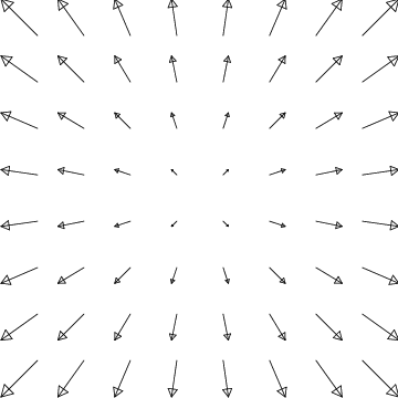
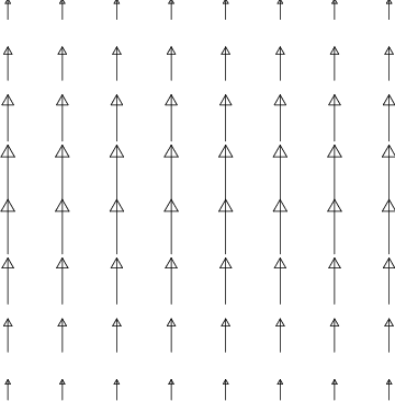
Which of the vector fields in Figure 9.10.1 is conservative?

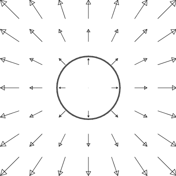
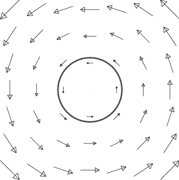
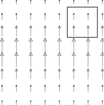
It is usually easy to determine that a given vector field is not conservative: Simply find a closed path around which the circulation of the vector field doesn’t vanish. But how does one show that a given vector field is conservative? Consider the vector fields in Figure 9.10.2. It is easy to see that the figure on the right is not conservative. But what about the one on the left?

Figure 9.10.2. The same two vector fields, with loops.

Figure 9.10.2. The same two vector fields, with loops.

A conservative vector field is the gradient of a potential function. The “equipotential” surfaces, on which the potential function is constant, form a topographic map for the potential function, and the gradient is then the slope field on this topo map. This analogy is exact for functions of two variables; conservative vector fields are those which correspond to topo maps.

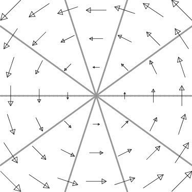
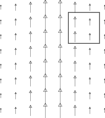
This fact provides a graphical technique for determining whether a given vector field (in two dimensions) is conservative: Try to draw its topo map. Let’s give it a try. Yes indeed, the vector field on the left in Figure 9.10.3 appears to be conservative, and the one on the right is not. What are the rules?

The level curves must be everywhere perpendicular to the vector field.
The level curves must be close together where the magnitude of the vector is large.
Level curves corresponding to different values may not intersect.

Figure 9.10.3. The same two vector fields, with level curves.

Figure 9.10.3. The same two vector fields, with level curves.

Here are two more examples. Which of the vector fields in Figure 9.10.4 is conservative?

Figure 9.10.4. Two more vector fields.

Figure 9.10.4. Two more vector fields.

Try drawing boxes, as shown in Figure 9.10.5.

Figure 9.10.5. The same two vector fields, with loops

Figure 9.10.5. The same two vector fields, with loops

Try drawing level curves, as shown in Figure 9.10.6.

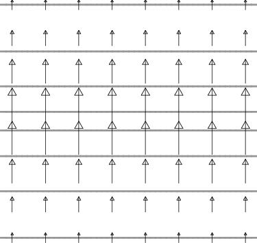
Figure 9.10.6. The same two vector fields, with level curves

Figure 9.10.6. The same two vector fields, with level curves

What can you conclude?